Analysis of Algorithms

Analysis of Algorithms#

Problem?

a task to be performed
best thought in terms of (well-defined) inputs and outputs
problem definition does not impose constraints on how the problem is solved but often includes resource constraints

Algorithm?

a sequence of steps followed to solve a problem
it must be correct and composed of a finite number of concrete steps
there can be no ambiguity
it must terminate

Program?

a representation of an algorithm in some programming language

Analysis of algorithms#

Algorithms

“Any well-defined computational procedure that takes some value, or set of values, as input and produces some value, or set of values, as output.”

—[Cormen et al., Introduction to Algorithms, 3rd.Ed.]

Resources necessary to execute an algorithm?

Time Complexity (running time)
Space Complexity (memory)

Resources typically depend on input size

Developing a usable algorithm#

The building blocks of algorithms

An algorithm is a step by step process that describes how to solve a problem in a way that always gives a correct answer. When there are multiple algorithms for a particular problem (and there often are!), the best algorithm is typically the one that solves it the fastest.

As computer programmers, we are constantly using algorithms, whether it’s an existing algorithm for a common problem, like sorting an array, or if it’s a completely new algorithm unique to our program. By understanding algorithms, we can make better decisions about which existing algorithms to use and learn how to make new algorithms that are correct and efficient. An algorithm is made up of three basic building blocks: sequencing, selection, and iteration.

– Khan Academy

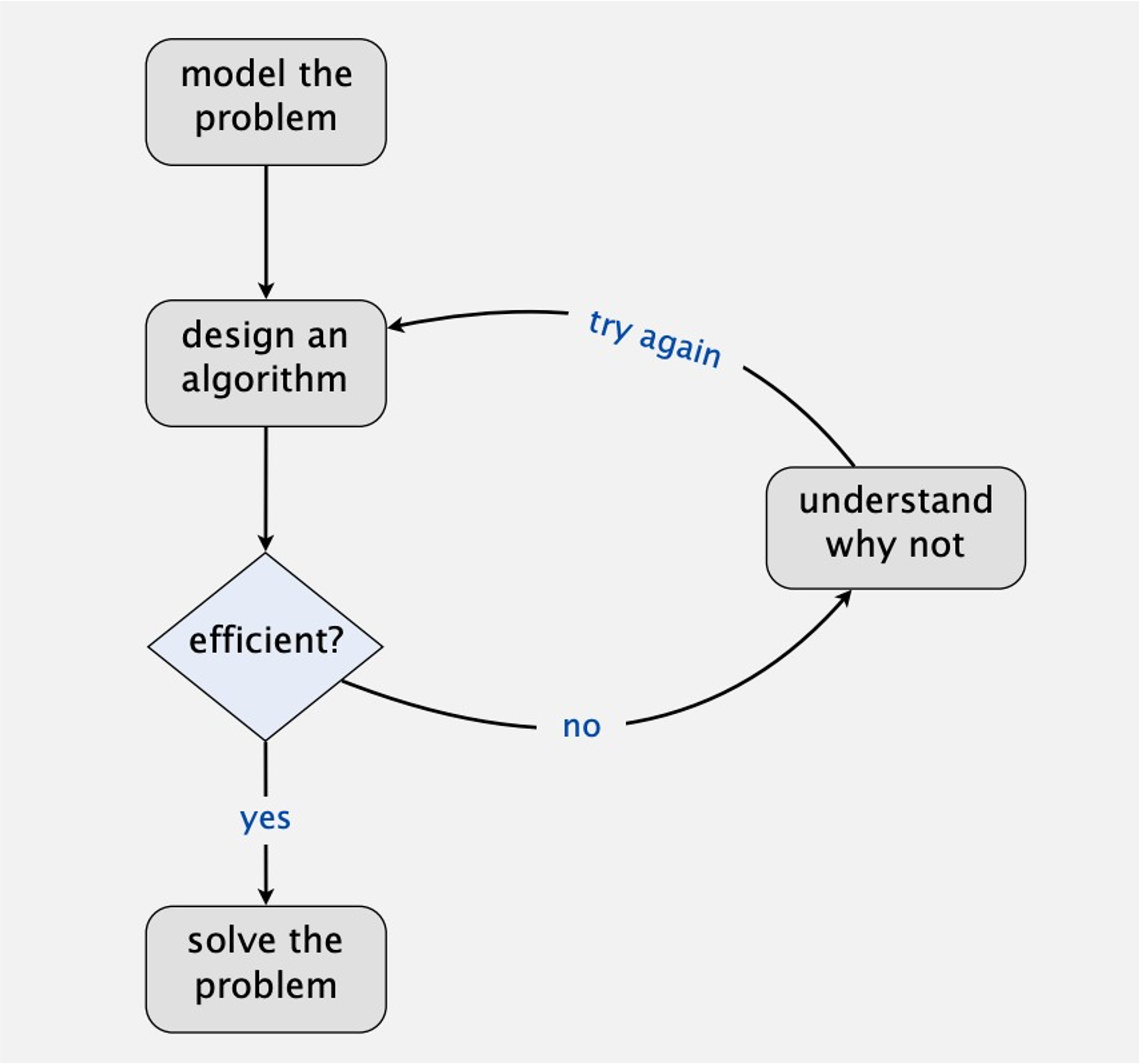
../../_images/w1_algo_design.png — Fig. 87 COS 226 lectures, Princeton University#

Sequencing: An algorithm is a step-by-step process, and the order of those steps are crucial to ensuring the correctness of an algorithm.

– Khan Academy

Selection: Algorithms can use selection to determine a different set of steps to execute based on a Boolean expression.

– Khan Academy

Iteration: Algorithms often use repetition to execute steps a certain number of times or until a certain condition is met.

– Khan Academy

Example from CS50

Why analyze algorithms?#

Classify algorithms/problems
Predict performance/resources
Provide guarantees
Understand underlying principles of problems
and…

../../_images/w3_01.png — Fig. 88 What do these all have in common?#

Analyzing computational cost#

Empirical Model

Run algorithm
Measure actual time

Mathematical Model

Analyze algorithm
Develop Model

Empirical analysis (timing)#

Implement algorithm
Run on different input sizes
Record actual running times
Calculate hypothesis
Predict and validate

Timing Algorithms#

Example 1

Euler’s Number

… mathematical constant that is the base of the natural logarithm. It is approximately equal to 2.71828.

\(e\)

\[\begin{split} \begin {align} e & = \lim_{x\to \infty} \bigg(1 + \frac{1}{n} \bigg)^n \\ & = \frac{1}{0!} + \frac{1}{1!} + \frac{1}{2!} + \frac{1}{3!} + \frac{1}{4!} + \dotsb \\ & = 1 + \frac{1}{1} + \frac{1}{1 * 2} + \frac{1}{1 * 2 * 3} + \frac{1}{1 * 2 * 3 * 4} + \dots + \frac{1}{n!} \\ \end {align} \end{split}\]

Leonhard Euler (1707–1783)

https://personajeshistoricos.com/wp-content/uploads/2018/04/Leonhard-Euler-2-785x1024.jpg — Fig. 89 a Swiss mathematician, physicist, astronomer, geo grapher, logician and engineer who made important and influential discoveries in many branches of mathematics.#

visualizations

Algorithms#

Which is more efficient?

Algorithm 1

long double euler1 (int n) {
    long double sum = 0;
    long double fact;
    for (int i = 0; i <= n; i++) {
        fact = 1;
        for (int j = 2; j <= i; j++) {
            fact *= j; 
        }
        sum += (1.0/fact);
    }
    return sum;
}

Algorithm 2

long double euler2 (int n) {
    long double sum = 0;
    long double fact = 1;
    for (int i = 0; i <= n; i++) {
        sum += (1.0/fact);
        fact *= (i + 1); 
    }
    return sum;
}

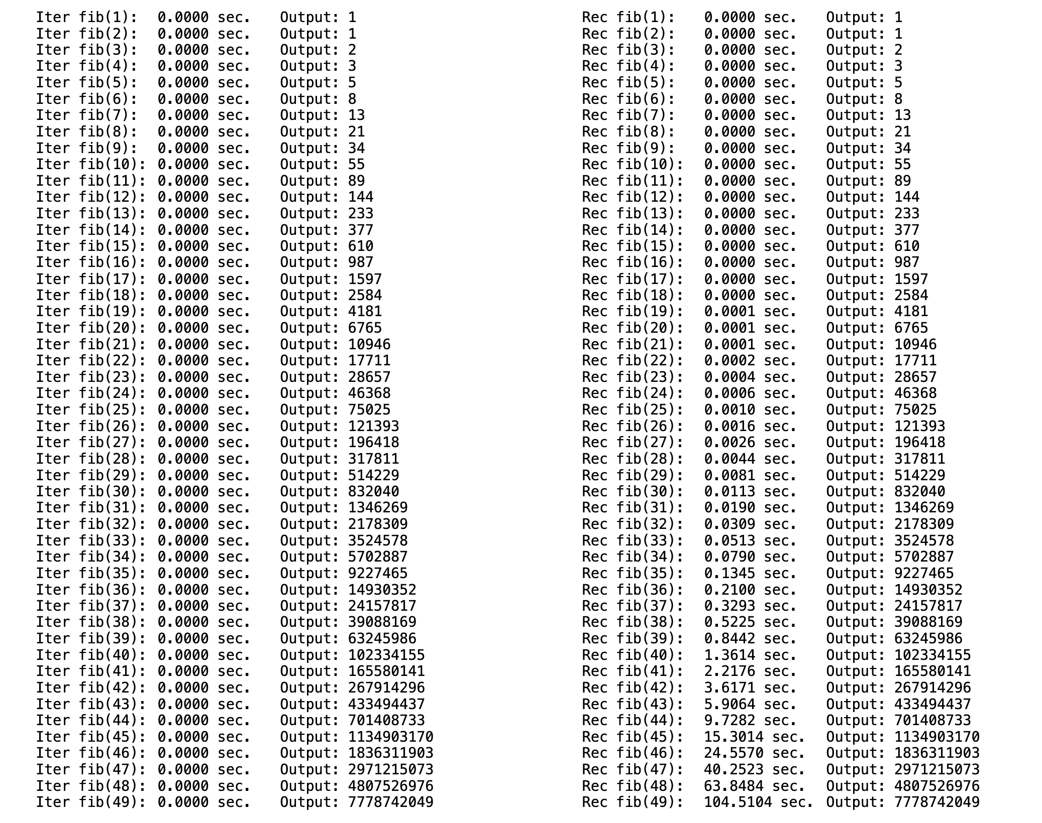
Example 2

https://azcoinnews.com/wp-content/uploads/2019/11/1-8.jpg — Fig. 90 fibonacci#

recurrence relation

\[\begin{split} F_0 & = 0 \\ F_1 & = 1 \\ F_n & = F_{n-1} + F_{n-2} \\ & = 0, 1, 1, 2, 3, 5, 8, 13, 21, 34 \dotsb \end{split}\]

Iterative

uint64_t fibI(uint16_t n){
    uint64_t sum;
    uint64_t prev[] = {0,1};
    if (n < 2) return n;
    for (uint16_t i = 2; i <= n; i++) {
        sum = prev[0] + prev[1];
        prev[0] = prev[1];
        prev[1] = sum;
    }
    return sum;
}

Recursive

uint64_t fibR (uint16_t n) {
    if (n < 2) return n;
    else return fibR(n-1) + fibR(n-2);
}

Timing…

void time_func(uint16_t n, const char *name) {
    uint64_t val;
    Clock::time_point tic,toc;
    if (! strcmp(name,"Iter")) {
        tic = Clock::now();
        val = fib_iter(n);
        toc = Clock::now();
    }
    if (! strcmp(name,"Rec")) {
        tic = Clock::now();
        val = fib_rec(n);
        toc = Clock::now();
    }
    std::cout << name << "fib(" << n << "):\t" 
              << std::fixed << std::setprecision(4) 
              << Seconds(toc-tic).count() << "sec.\tOutput:"
              << val << std::endl; 
}
    
int main (int argc, char** argv) {
    if (argc != 3) {
        std::cout << "Usage:./fib<n><alg>\n";
        std::cout << "\t<n>\tn-th term to be calculated\n";
        std::cout << "\t<alg>\t algorithm to be used(RecorIter)\n";
        return 0;
    }
    uint16_t n = (uint16_t)
    atoi(argv[1]);
    time_func(n,argv[2]);
}

Outcomes

../../_images/w3_02.png — Fig. 91 Iterative v. Recursive#

Is this as expected?

Hypothesis

../../_images/w3_03.png — Fig. 92 graph#

Complete the graph, what would it look like?

Limitations of empirical analysis#

Requires implementing several algorithms for the same problem

may be difficult and time consuming
implementation details also play a role (one particular algorithm may be “better written”)

Requires extensive testing

time consuming
choice of test cases might favor one of the algorithms

Variations in hardware, software, and operating system affect analysis