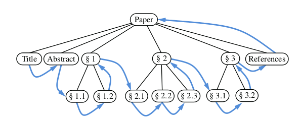
Binary Search Trees

Binary Tree

Overview

• A binary tree is a hierarchical data structure consisting of nodes.

• Each node contains a value and references to its left and right children.

• The left child is smaller than the parent, while the right child is larger.

\[bin\_tree = \{1, 7, 9, 2, 6, 9, 5, 11, 5 \}\]

Implementing binary trees

Node

\(data\)

\(left\) child

\(right\) child

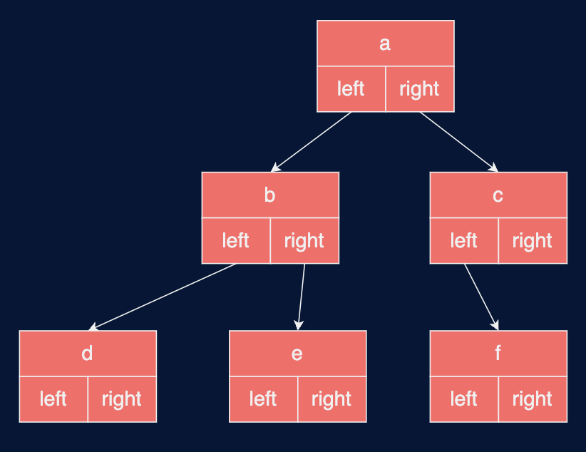
\(tree = \{a, b, c, d, e, f\}\)

\(k\)-ary trees

k-ary trees

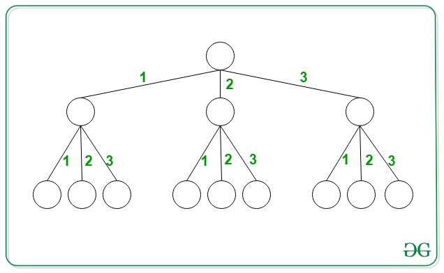
Fig. 14 Every node has between \(0\) and \(k\) children

types

full

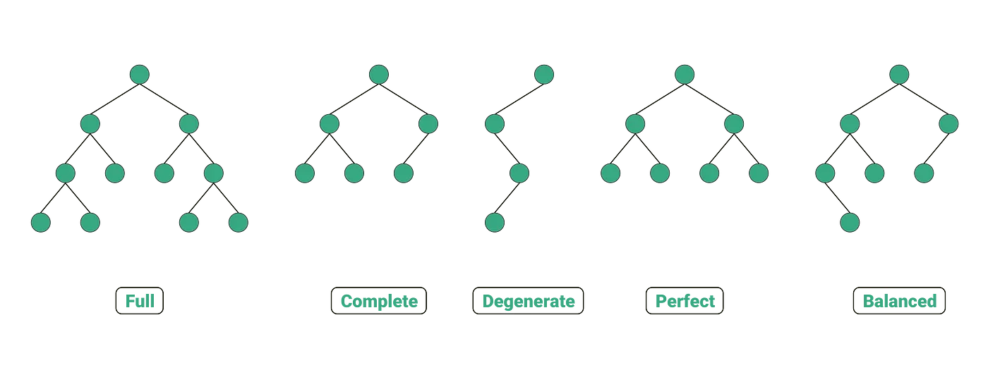
Fig. 15
Full Binary Tree is a Binary Tree in which every node has 0 or 2 children.
– towardsdatascience.com

complete

Fig. 16
Complete Binary Tree has all levels completely filled with nodes except the last level and in the last level, all the nodes are as left side as possible. – towardsdatascience.com

perfect

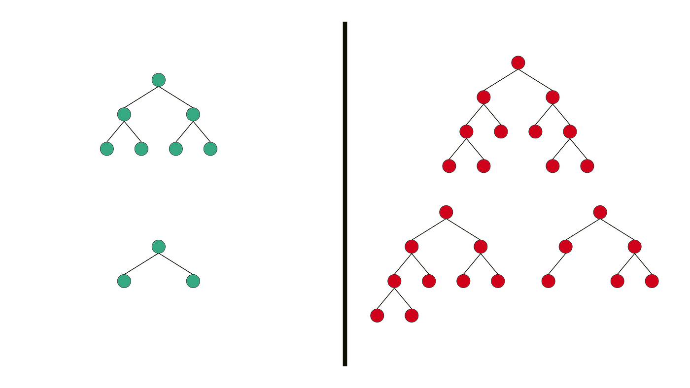
Fig. 17
Perfect Binary Tree is a Binary Tree in which all internal nodes have 2 children and all the leaf nodes are at the same depth or same level. – towardsdatascience.com

degenerate

Fig. 18
Degenerate Binary Tree is a Binary Tree where every parent node has only one child node. – towardsdatascience.com

balanced

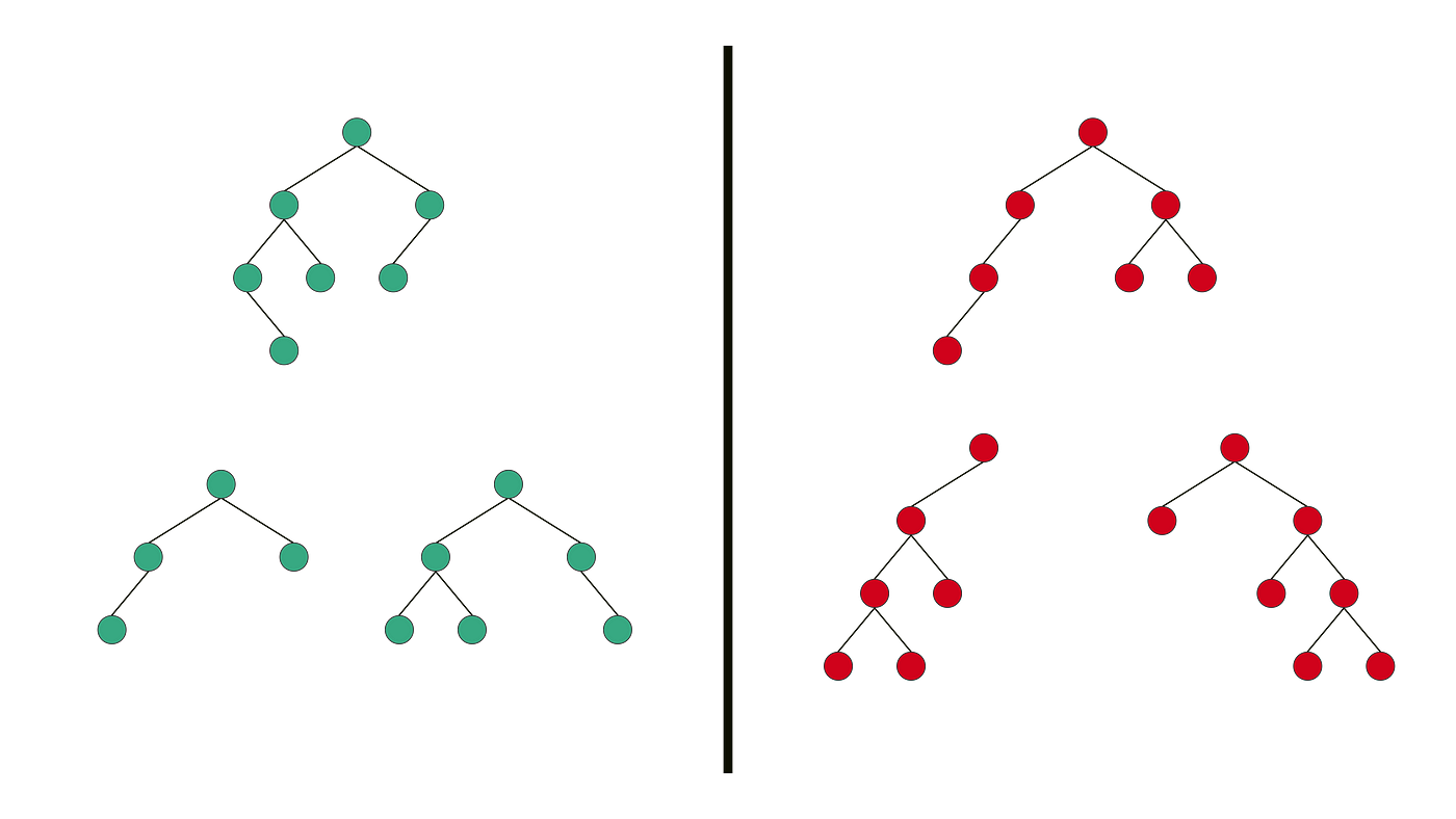
Fig. 19
Balanced Binary Tree is a Binary tree in which height of the left and the right sub-trees of every node may differ by at most 1. – towardsdatascience.com

Binary Search Trees

Understanding BSTs

• Each node in a binary tree can have at most two children.

  • This means that a node can have either zero, one, or two children.

• The left child of a node is typically smaller than the node, while the right child is larger (or equal) than the node.

  • This rule is often associated with binary search trees (BSTs), where the values are arranged in a specific order for efficient searching and retrieval.

• The order of children matters.

  • In a binary tree, the left child is typically referenced before the right child.

  • The order of children affects the tree’s traversal and interpretation.

• Nodes are connected by edges.

  • The connections between nodes are represented by edges in a binary tree.

  • Each node (except the root) has exactly one incoming edge from its parent.

• The height of a binary tree.

  • The height of a binary tree is the maximum number of edges from the root to a leaf node.

  • It represents the longest path from the root to any leaf node in the tree.

• The depth (level) of a node.

  • The depth (or level) of a node in a binary tree represents the number of edges from the root to that node.

  • The root node is at depth 0, its children are at depth 1, and so on.

• The number of nodes in a binary tree.

  • The total number of nodes in a binary tree can vary.

  • The minimum number of nodes in a binary tree is 0, while the maximum number depends on the height of the tree.

Simplified is bst

A BST has symmetric order

• each node \(x\) in a BST has a key

\[key(x)\]

• for all nodes \(y\) in the left subtree of \(x\),

\[key(y) < key(x)^{**}\]

• for all nodes \(y\) in the right subtree of \(x\),

\[key(y) > key(x)^{**}\]

Example

(**) assume that the keys of a BST are pairwise distinct

Tree Parts

BST Classes

BSTNode

class BSTNode { 
  
  private: 
    int data;  
    BSTNode *left;  
    BSTNode *right;
  
  public:
    BSTNode(int d);
    ~BSTNode();
  
  friend class BSTree;

};

BSTree

class BSTree{
  
  private:
    BSTNode *root;
    void destroy(BSTNode *p);
    
  public:
    BSTree();
    ~BSTree();
    void insert(int d);
    void remove(int d);  
    BSTNode *search(int d);

};

search

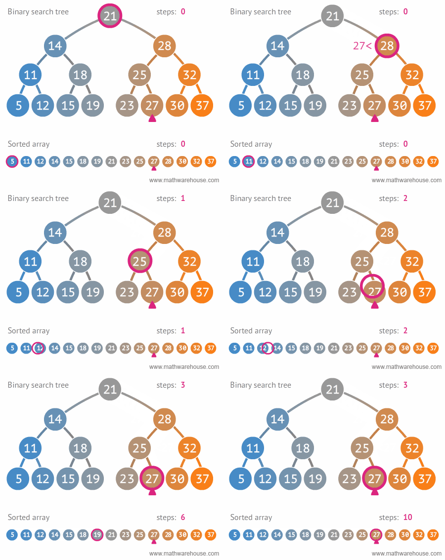
1. Start at root node

2. If the search key:
   a. matches the current node’s key
   * then found
   b. If search key \(>\) current node’s key
   * search on \(right\) child
   c. If search key is less than current node’s
   * search on \(left\) child

3. Stop when current node is NULL (not found)

\(Search\ for\ \ 8\)

visualize

try it

insert

To insert a new value into a BST:

• Start at the root node.

• If the value is smaller, go to the left subtree; if larger, go to the right subtree.

• Repeat steps 2 until an empty spot is found.

• Insert the new node in the empty spot.

visualize

try it

remove

To delete a node from a BST:

• Find the node to delete.

• If the node has no children, simply remove it.

• If the node has one child, replace it with its child.

• If the node has two children, find the node’s successor (smallest value in the right subtree) or predecessor (largest value in the left subtree).

• Replace the node with its successor/predecessor and delete the successor/predecessor from its original position.

leaf

Fig. 20 \(remove : leaf\)

1 child

Fig. 21 \(remove:\ with\ 1\ child\)

2 children

Fig. 22 \(remove:\ with\ 2\ children\)

visualize

try it

Traversals

Implications

Traversal of a tree T is a systematic way of accessing, or “visiting,” all the positions of T . The specific action associated with the “visit” of a position p depends on the application of this traversal, and could involve anything from incrementing a counter to performing some complex computation for p.

preorder

// nodes of the BST are visited in a
// pre-defined order before visiting
// their child nodes.

algorithm preorder (p) {
  if (p) {
    visit(p)
    preorder(p -> left)
    preorder(p -> right)
  }
}

Fig. 23 preorder

animation

try it

postorder

// nodes of the BST are visited in a 
// pre-defined order after visiting 
// their child nodes.

algorithm postorder (p) {
  if (p) {
    postorder(p -> left)
    postorder(p -> right)
    visit(p)
  }
}

Fig. 24 postorder

animation

try it

inorder

// nodes of the BST are visited in
// ascending order of their values.

algorithm inorder (p) {
  if (p) {
    inorder(p -> left)
    visit(p)
    inorder(p -> right)
  }
}

Fig. 25 inorder

animation

How would we:

Destroy a binary tree

Post Order

Fig. 26
Post Order

Why?

It’s the only traversal that visits all the subtree nodes before visiting the root. All child nodes must be removed before we can delete the root.

Print all elements ascending order

In Order

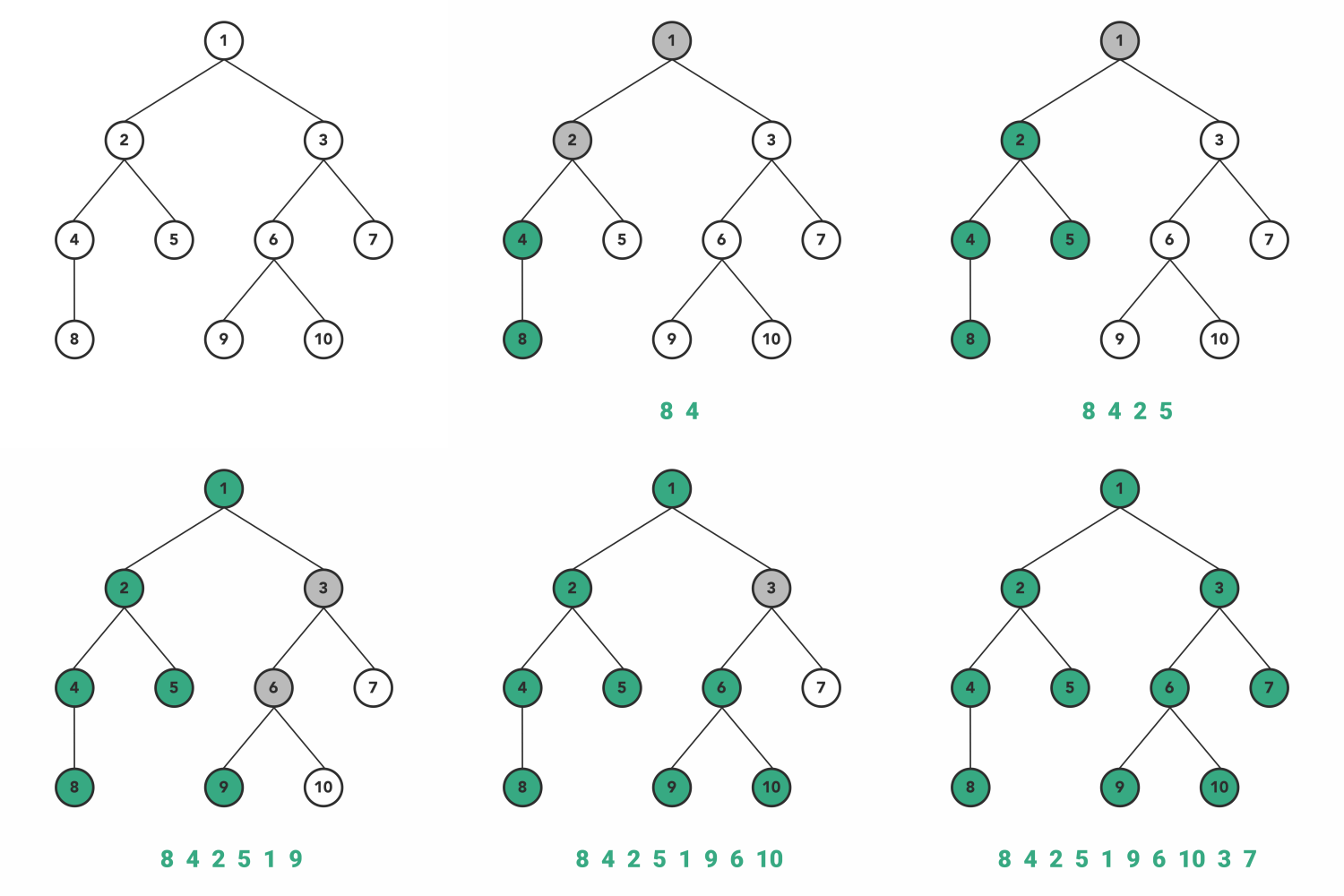
Why?

to output in ascending order, we would need to start with the lowest value sequentially and work our way to the largest; as BST’s are built in sequential order, \(in-order\) fits best

incomplete

	best-case	worst-case	average-case
search
insert
remove

\[Cost\ of\ basic\ operations??\]

complete

	best-case	worst-case	average-case
search	\(O(1)\)	\(O(n)\)	\(O(log\ n)\)
insert	\(O(1)\)	\(O(n)\)	\(O(log\ n)\)
remove	\(O(log\ n)\)	\(O(n)\)	\(O(log\ n)\)

\[Cost\ of\ basic\ operations??\]

Average-case analysis

If \(n\) distinct keys are inserted into a BST in random order, expected number of compares for basic operations is

\[\ \sim2\ ln\ n \approx 1.39\ log\ n\ \]

• proof: 1-1 correspondence with quick-sort

\[ \ \ h = O(log\ n) \ \ \]

inserting n keys in a random order

\(n = 255\)

Fig. 27 https://algs4.cs.princeton.edu/32bst/

Collections / Dictionaries

	What?	Sequential (unordered)	Sequential (ordered)	BST
search	search for a key	\(O(n)\)	\(O(log\ n)\)	\(O(h)\)
insert	insert a key	\(O(n)\)	\(O(n)\)	\(O(h)\)
delete	delete a key	\(O(n)\)	\(O(n)\)	\(O(h)\)
min/max	smallest/largest key	\(O(n)\)	\(O(1)\)	\(O(h)\)
floor/ceiling	predecessor / successor	\(O(n)\)	\(O(log\ n)\)	\(O(h)\)
rank	# of keys less than key	\(O(n)\)	\(O(log\ n)\)	\(O(h)\)**

(**) requires the use of ‘size’ at every node