Big-O

Big-O#

The story so far…#

Can measure actual runtime to compare algorithms

however, runtime is noisy (highly sensitive to hardware/software and implementation details)

Can count instructions to compare algorithms

can define $T(n)$, which depends on the input size
for large inputs, our focus should be on the dominant terms of $T(n)$

Inline Math#

Sequence & Series

Sequence

also known as a progression, is a successive arrangement of numbers in an order according to some specific rules

– gfg

Depending upon the number of terms in a sequence, it is classified into two types, namely a finite sequence and an infinite sequence.

examples

finite arithmetic sequence: $3, 5, 7, 9, 11$
infinite geometric sequence: $2, 4, 8, 16, …… $

Series

formed by adding the elements of a sequence

– gfg

Depending on whether the sequence is finite or infinite, the series can be either finite or infinite.

examples

finite arithmetic series: $3 + 5 + 7 + 9 + 11$
infinite geometric series: $2 + 4 + 8 + 16 + …… $

Arithmetic

Arithmetic Sequence and Series

where each term of the sequence is formed either by adding or subtracting a common term from the preceding number

$2, 5, 8, 11, 14,…$

Geometric

Geometric Sequence and Series

where each term of the sequence is formed either by multiplying or dividing a common term with the preceding number

$1, 5, 25, 125, 625,…$

Harmonic

Harmonic Sequence and Series

where each term of the sequence is the reciprocal of the element of an arithmetic sequence

$2, 5, 8, 11, 14,…$

Fibonacci

Fibonacci Numbers

a sequence of numbers where each term of the sequence is formed by adding its preceding two numbers, and the first two terms of the sequence are 0 and 1

\[\begin{split} \begin {align} F_0 & = 0 \\ F_1 & = 1 \\\ F_2 & = F_1 - F_0 \\\ & = 1 + 0 \\\ & = 1 \\\ F_3 & = F_2 + F_1 \\\ & = 1 + 1 \\\ & = 2 \\ \end {align} \end{split}\]

Sigma Notation

https://i.pinimg.com/736x/df/35/19/df351990b77146392f2c8b3b0ab9681c--algebra--math-resources.jpg — Fig. 93 sigma notation#

Summation Formulas

general premise: $\sum_{i = 1}^{n} 1 = n$

geometric sequence

for $a, ar, ar^2, ... , ar^{n - 1}$

function sum_of_geometric_sequence(first_term, common_ratio, n):
    if n <= 0:
        return 0
    else:
        sum = 0
        term = first_term
        for i from 1 to n do:
            sum = sum + term
            term = term * common_ratio
        return sum

sum of the first n terms $$ \begin {align} \Longrightarrow \sum_{i = 1}^{n} ar^{i - 1} = \frac{a(1 - r^n)}{1 - r} \\ \end {align} $$

Explanation

This pseudocode defines a function sum_of_geometric_sequence that takes three parameters: first_term, common_ratio, and n. first_term represents the first term of the geometric sequence. common_ratio represents the common ratio between consecutive terms of the sequence. n represents the number of terms you want to sum. It first checks if n is less than or equal to 0. If n is 0 or negative, it returns 0 because the sum of 0 terms in any sequence is 0. If n is greater than 0, it initializes a variable sum to 0 to keep track of the running sum and a variable term to first_term to represent the current term of the sequence. It then uses a for loop to iterate from 1 to n, adding the current term to the sum in each iteration. After adding the term to the sum, it updates the term by multiplying it by the common_ratio to get the next term in the sequence. The loop continues until n terms have been added to the sum, and then the function returns the final value of sum.

$sum = \frac{first_term}{1 - common}$

function sum_of_infinite_geometric_series(first_term, common_ratio):
    if abs(common_ratio) >= 1:
        # The series diverges if the common ratio is greater than or equal to 1.
        return "Divergent (sum does not exist)"
    else:
        # Calculate the sum using the formula.
        sum = first_term / (1 - common_ratio)
        return sum

sum of the infinite terms $$ \begin {align} \Longrightarrow \sum_{i = 1}^{n} ar^{i - 1} = \frac{a}{1 - r}$, only when $|r| \lt 1 \end {align} $$

Explanation

This pseudocode defines a function sum_of_infinite_geometric_series that takes two parameters: first_term and common_ratio. first_term represents the first term of the geometric series. common_ratio represents the common ratio between consecutive terms of the series. It first checks if the absolute value of common_ratio is greater than or equal to 1. If the common ratio is greater than or equal to 1, the series diverges, and the function returns “Divergent (sum does not exist)” because the sum does not exist in such cases. If the common ratio is less than 1, it calculates the sum using the formula mentioned earlier and returns the result.

Sigma Ex 1

Summation of the first N Integers : $\sum_{i = 1}^n i$

int main() {
  int i, sum = 0, n;
  scanf("%d", &n);

  for(i=1; i<=n; i++) {
    sum = sum + i;
  }

  printf("%d", sum);
  return 0;
}

Sigma Ex 2

Summation Two Power : $\sum_{i = 0}^{n} 2^i$

Comparing Algorithms#

Comparative rules

\[\begin{split}\begin{align} 1. log\ ab &= log\ a + log\ b \\ 2. log\ \frac{a}{b} &= log\ a - log\ b \\ 3. log\ a^b &= b\ log\ a \\ 4. a^{log^{b}_{c}} &= b^{log^{a}_{c}} \\ 5. a^b &= n \Longrightarrow b = log_a\ n \end{align}\end{split}\]

1.10.1 Comparison of Functions #1
1.10.2 Comparison of Functions #2

Compare two…

$Are\ these\ the\ same?$

\[\color{green}{T(n) = 2n} \ \ \ \ \ \ \ \ \color{orange}{T(n) = 25n}\]

Smaller datasets...

Larger datasets...

\[Why\ / Why\ Not?\]

Explanation

Looking closely at the graphs, the left graph has low input ($n$) values…when we look to the right and reveal the graph for high input ($n$) values, the behavior of the lines on the graph remains the same. Therefore the algorithms themselves are the same…

Compare three…

$Are\ these\ the\ same?$

\[\color{green}{T(n) = 2n} \ \ \ \ \ \ \ \ \color{orange}{T(n) = 25n} \ \ \ \ \ \ \ \ \color{blue}{T(n) = n^2}\]

Smaller datasets...

Larger datasets...

Largest datasets...

\[Why\ / Why\ Not?\]

Explantion

Looking closely at the graphs, the left graph has low input ($n$) values…when we look to the right and reveal the graph for high input ($n$) values, the behavior of the lines on the graph remains the same. Therefore the algorithms themselves are the same…

Compare two more…

$Are\ these\ the\ same?$

\[\color{green}{T(n) = 1000n + 500} \ \ \ \ \ \ \ \ \color{orange}{T(n) = n^2}\]

Smaller datasets...

Larger datasets...

"Big Data"...

\[Why\ / Why\ Not?\]

Bottom line…

We are trying to compare $T(n)$ functions, but…

we also care about large values of $n$

Can we properly define $\le$ for functions?

we can group functions into $sets$ and make our lives easier

Asymptotic Analysis #

refers to the study of an algorithm as the input size “gets big” or reaches a limit (in the calculus sense)

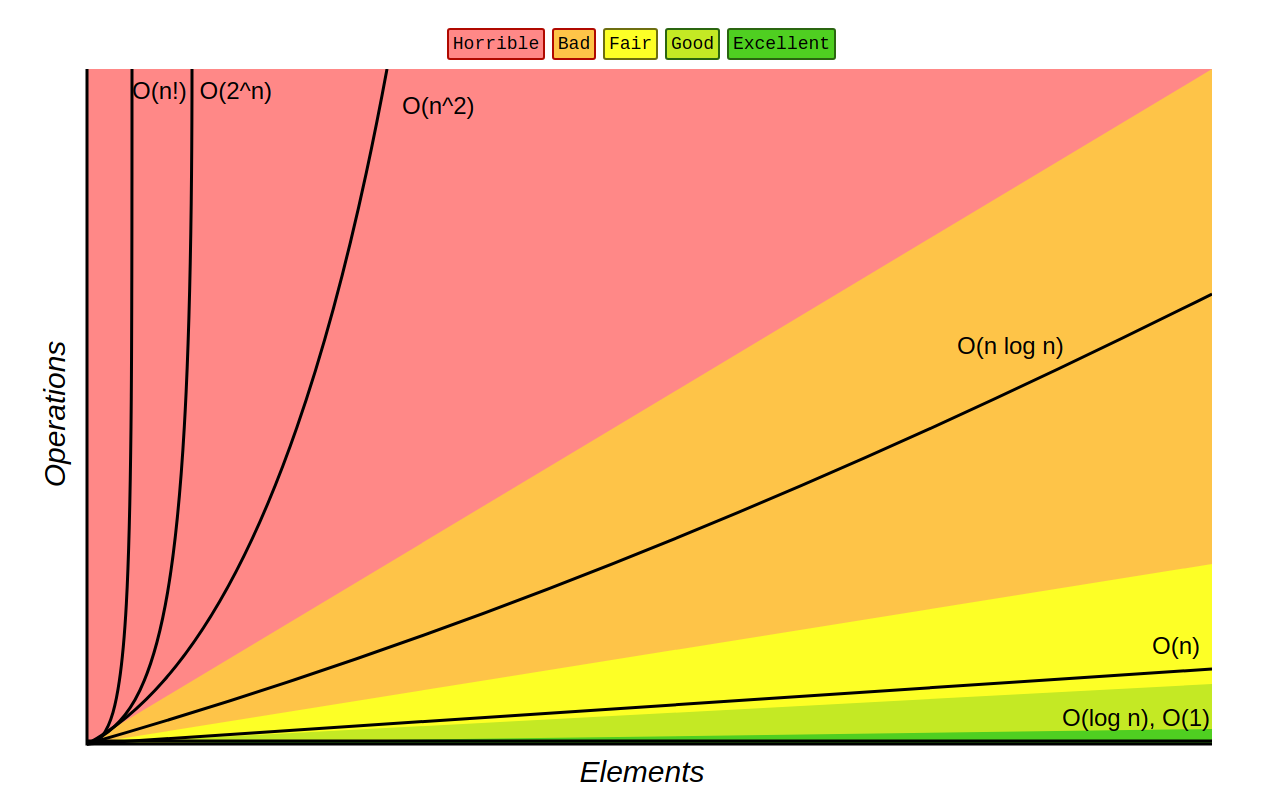
Growth rate#

rate at which the cost of an algorithm grows as the size of its input grows

\[c_1n\]

\[c_2n^2\]

Common sets of functions#

Algorithm $A$ is better than Algorithm $B$ if…

for large values of $n$, $TA(n)$ grows slower than $TB(n)$

Note: Faster growth rate…slower algorithm…

Examples#

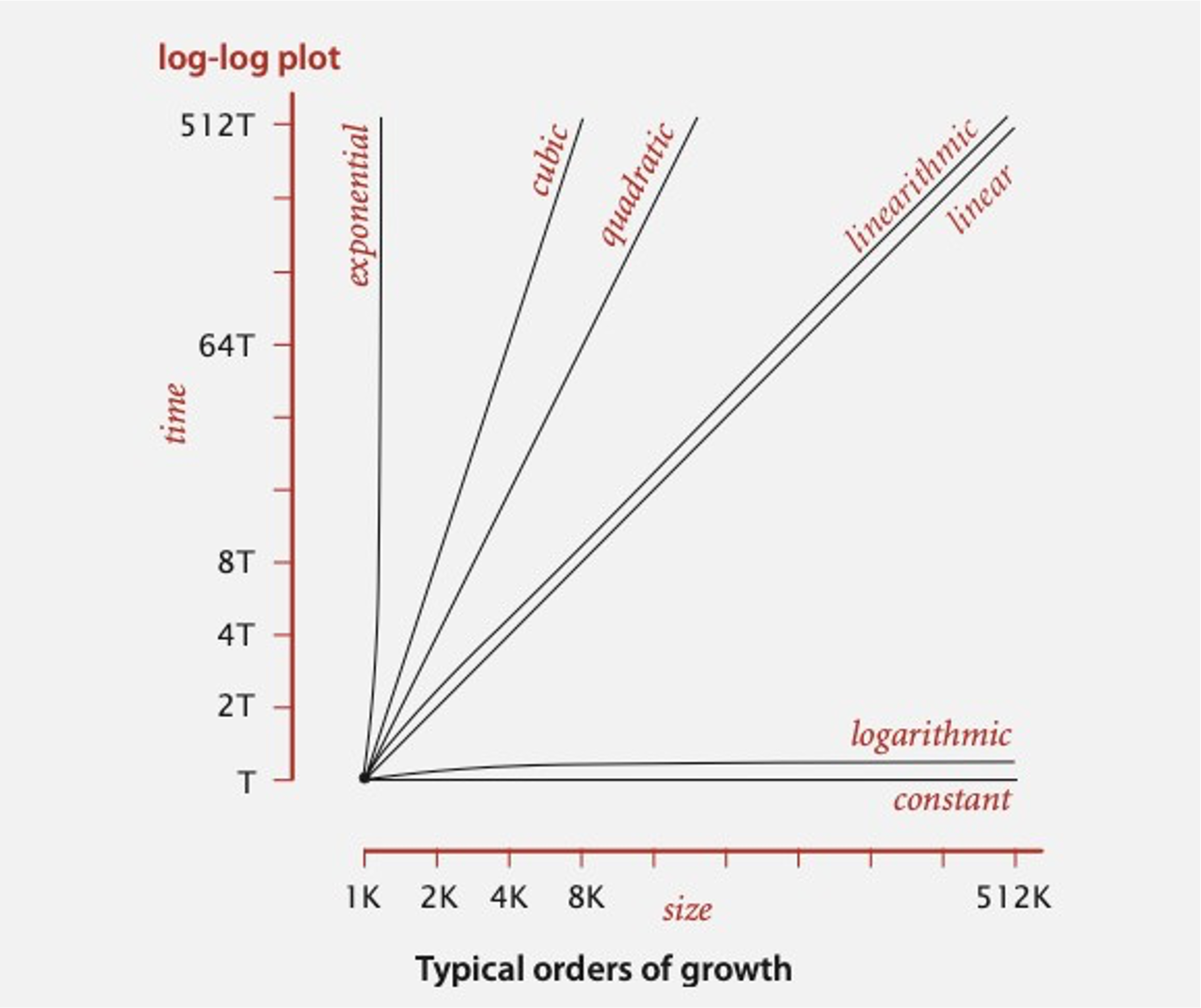
order of growth	name	typical code framework	description	example
\[1\]	constant	\[a = b + c;\]	statement	add two numbers
\[log\ n\]	logarithmic	\[\begin{split}while\ (n > 1)\\ \{ \ \ \ \ \ \ \ \dots \ \ \ \ \ \ \ \}\end{split}\]	divide in half	binary search
\[n\]	linear	\[\begin{split}for\ (int\ i\ = 0; i \lt n; i++)\\ \{ \ \ \ \ \ \ \ \dots \ \ \ \ \ \ \ \}\end{split}\]	single loop	find the maximum
\[n\ log\ n\]	linearithmic	\[see\ mergesort\]	divide & conquer	mergesort
\[n^2\]	quadratic	\[\begin{split}for\ (int\ i\ = 0; i \lt n; i++)\ \ \ \ \ \ \ \ \ \ \ \ \ \ \ \ \ \ \\ for\ (int\ j\ = 0; j \lt n; j++)\ \ \ \ \ \ \ \ \ \\ \ \ \ \ \ \ \ \ \{ \ \ \ \ \ \ \ \dots \ \ \ \ \ \ \ \}\end{split}\]	double loop	check all pairs
\[n^3\]	cubic	\[\begin{split}for\ (int\ i\ = 0; i \lt n; i++)\ \ \ \ \ \ \ \ \ \ \ \ \ \ \\ for\ (int\ j\ = 0; j \lt n; j++)\ \ \ \ \ \ \ \ \ \\ \ \ \ \ for\ (int\ k\ = 0; k \lt n; k++)\\ \{ \ \ \ \ \ \ \ \dots \ \ \ \ \ \ \ \}\end{split}\]	double loop	check all pairs
\[2^n\]	exponential	\[see\ combinatorial\ search\]	exhaustive search	check all subsets

Asymptotic Bounds#

Defined

Asymptotic bounds are a way of describing the behavior of an algorithm as the input size approaches infinity. They are used to analyze the time and space complexity of algorithms, and are expressed in terms of upper and lower bounds.

The most commonly used asymptotic bounds are Big-O notation, Omega notation, and Theta notation.

Big-O notation is an upper bound on the growth rate of an algorithm. It describes the worst-case scenario of an algorithm’s time complexity.
- Ex : if an algorithm has a time complexity of $O(n^2)$, it means that the running time of the algorithm grows no faster than $n^2$.
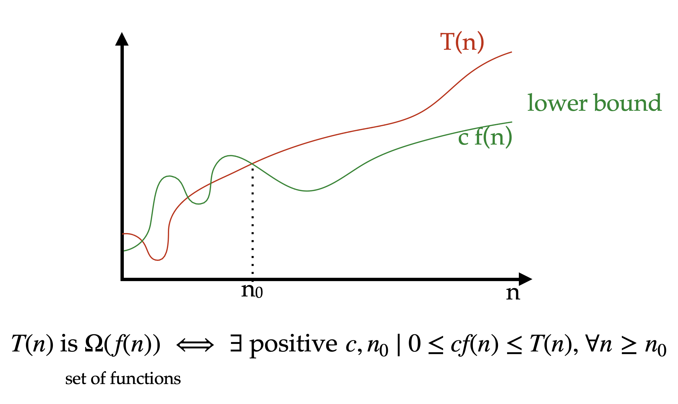
Big-Omega notation is a lower bound on the growth rate of an algorithm. It describes the best-case scenario of an algorithm’s time complexity.
- Ex. if an algorithm has a time complexity of $\Omega(n)$, it means that the running time of the algorithm grows at least as fast as $n$.
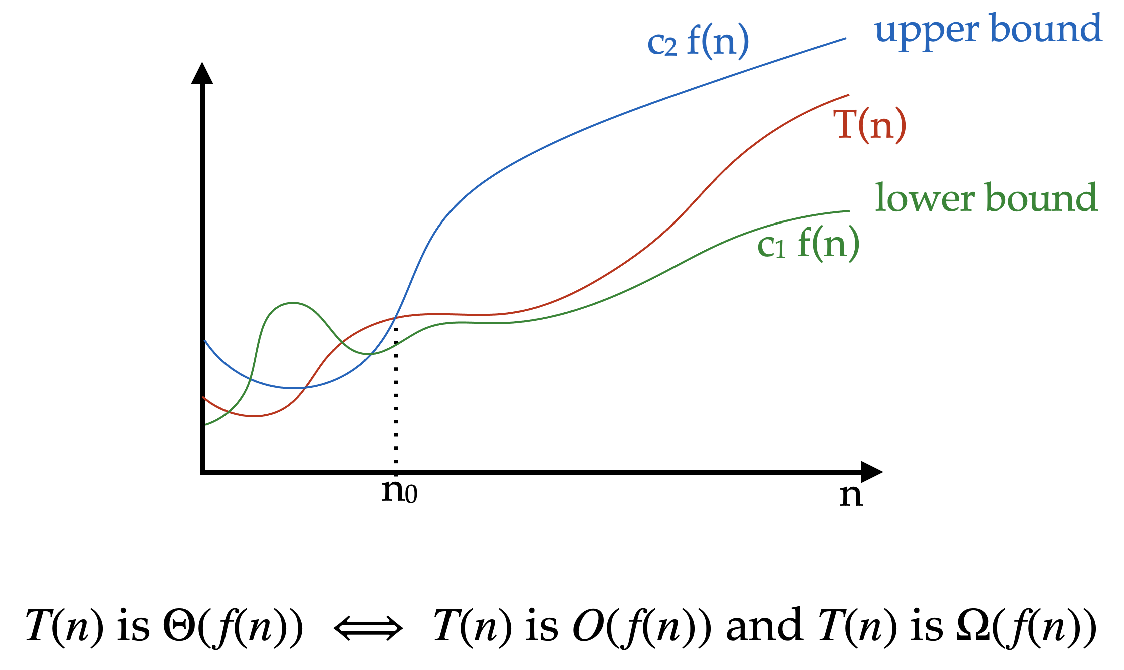
Theta notation provides both an upper and lower bound on the growth rate of an algorithm. It describes the tight bound on the growth rate of an algorithm.
- Ex. if an algorithm has a time complexity of $\Theta(n^2)$, it means that the running time of the algorithm grows exactly as fast as $n^2$.

Asymptotic bounds are useful because they allow us to compare the efficiency of different algorithms and to choose the most appropriate one for a given task.

Big-O

Definition

Translation

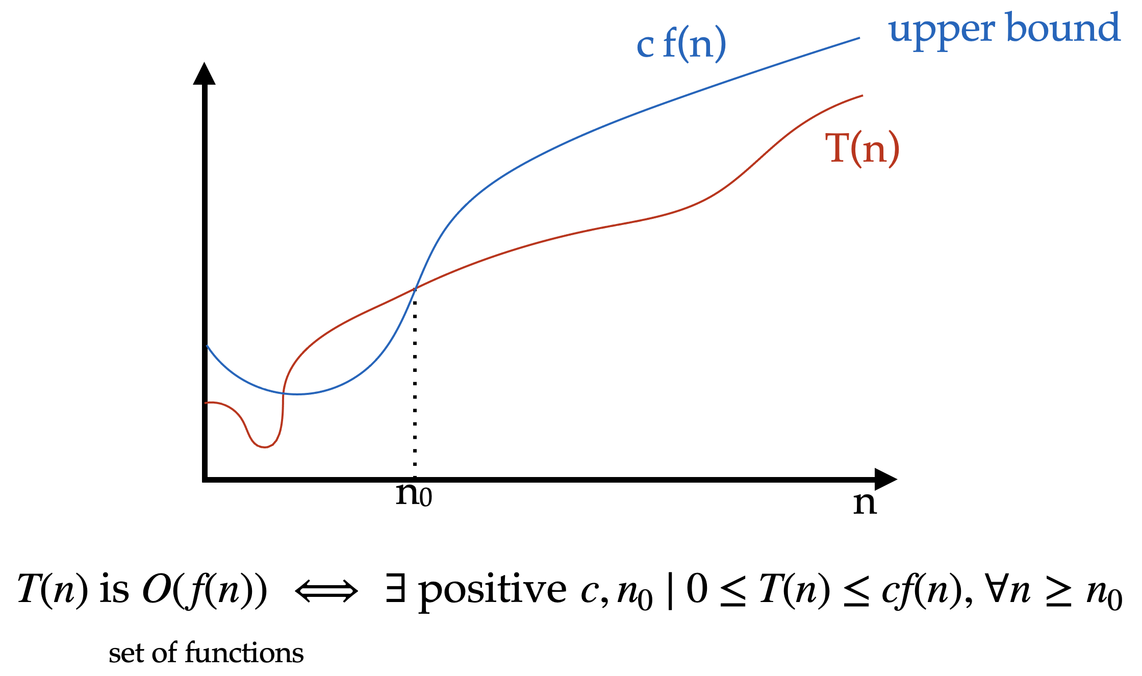
$T$ of $n$ is upper bounded by $F$ of $n$ if and only if $T$ of $n$ is less than or equal to some constant $C$ times $F$ of $n$ the function we chose to bound with for all $N$ greater than the initial $n$ or and not

Example

\[\begin{split}\begin{align} c.g : f(n) & = 2n + 3 \\ 2n + 3 & \le ?? \\ 2n + 3 & \le 10n \Longrightarrow O(n) \\ & alternatively, \\ 2n + 3 & \le 5n^2 \Longrightarrow O(n^2) \\ \end{align}\end{split}\]

Miscellaneous Notations

Big-Omega

Definition

Example

\[\begin{split}\begin{align} c.g :& f(n) = 2n + 3 \\ 2n + 3 & \ge 1 * n \ \ \ \forall n \le 1 \\ 2n + 3 & \ge n \Longrightarrow \Omega(n) \\ & alternatively, \\ 2n + 3 & \ge 1 * log\ n \ \ \ \forall n \le 1 \\ 2n + 3 & \ge 1 * log\ n \Longrightarrow \Omega(log\ n) \\ \end{align}\end{split}\]

Miscellaneous Notations

Theta

Definition

Example

\[\begin{split}\begin{align} c.g :& f(n) & = 2n + 3 \\ big-\Omega & \le 2n + 3 & \le big-\O \\ 1 * n & \le 2n +3 \le 5 * n \ \ \ \Longrightarrow \Theta(n) \\ \end{align}\end{split}\]

Miscellaneous Notations

Prove It

Proof of Theta

\[\begin{split}\begin{align} f(n) = 2n^2 + 3n + 4 & \\ & \Omega(n^2) \Longleftarrow 1 * n \ \ \ \ \ \ \ \le 2n^2 + 3n + 4 \le \ \ \ \ \ \ \ 9n^2 \Longrightarrow O(n^2) \\ & Therefore, \Theta(n^2) \\ \end{align}\end{split}\]

Proof of Theta

\[\begin{split}\begin{align} f(n) = n^2\ log\ n + n & \\ & \Omega(n^2\ log\ n) \Longleftarrow 1 * n^2\ log\ n \ \ \ \ \ \ \ \le n^2\ log\ n + n \le \ \ \ \ \ \ \ n^2\ log\ n \Longrightarrow O(n^2\ log\ n) \\ & Therefore, \Theta(n^2\ log\ n) \\ \end{align}\end{split}\]

Proof of No Theta

\[\begin{split}\begin{align} f(n) = n! & \\ & \Omega(1) \Longleftarrow 1 \ \ \ \ \ \ \ \le n! \le \ \ \ \ \ \ \ n^n \Longrightarrow O(n^n) \\ & Therefore, \Theta \ does\ not\ exist \\ \end{align}\end{split}\]

Proof of No Theta

\[\begin{split}\begin{align} f(n) = log\ n! & \\ & \Omega(1) \Longleftarrow 1 \ \ \ \ \ \ \ \le log\ n! \le \ \ \ \ \ \ \ log\ n^n \Longrightarrow O(n\ log\ n) \\ & Therefore, \Theta \ does\ not\ exist \\ \end{align}\end{split}\]

[1.8.2 Asymptotic Notations - Big Oh - Omega - Theta #2](https://youtu.be/Nd0XDY-jVHs?feature=shared)

In practice…#

“ignore constants and drop lower order terms”

Advantages & Disadvantages#

Advantages

Asymptotic analysis provides a high-level understanding of how an algorithm performs with respect to input size.

It is a useful tool for comparing the efficiency of different algorithms and selecting the best one for a specific problem.

It helps in predicting how an algorithm will perform on larger input sizes, which is essential for real-world applications.

Asymptotic analysis is relatively easy to perform and requires only basic mathematical skills.

– gfg

Disadvantages

Asymptotic analysis does not provide an accurate running time or space usage of an algorithm.

It assumes that the input size is the only factor that affects an algorithm’s performance, which is not always the case in practice.

Asymptotic analysis can sometimes be misleading, as two algorithms with the same asymptotic complexity may have different actual running times or space usage.

It is not always straightforward to determine the best asymptotic complexity for an algorithm, as there may be trade-offs between time and space complexity.

– gfg

True or False?#

\[Time\ Complexities:\ {1, log\ n, n, n\ log\ n, n^2, 2^n, n!}\]

Test yourself

Click near the center of a cell in each respective column to type your response…

	\[Big\ O\]	\[Big\ \Omega\]	\[\Theta\]
\[10^2 + 3000n + 10\]
\[21\ log\ n\]
\[500\ log\ n + n^4\]
\[\sqrt{n} + log\ n^{50}\]
\[4^n + n^{5000}\]
\[3000n^3 + n^{3.5}\]
\[2^5 +n!\]

Outcomes

	\[Big\ O\]	\[Big\ \Omega\]	\[\Theta\]
\[10^2 + 3000n + 10\]	\[\ge n\]	\[\le n\]	\[true\]
\[21\ log\ n\]	\[\ge log\ n\]	\[\le log\ n\]	\[true\]
\[500\ log\ n + n^4\]	\[\ge n^2\]	\[\le log\ n\]	\[false\]
\[\sqrt{n} + log\ n^{50}\]	\[\ge log\ n\]	\[\le log\ n\]	\[true\]
\[4^n + n^{5000}\]	\[\ge 2^n\]	\[\le n^2\]	\[false\]
\[3000n^3 + n^{3.5}\]	\[\ge n^2\]	\[\le n^2\]	\[true\]
\[2^5 +n!\]	\[\gt n!\]	\[\lt n!\]	\[false\]

Asymptotic Performance#

For $large$ values of $n$, a $Θ(n^2)$ algorithm always beats a $Θ(n^3)$ algorithm

However, we shouldn’t completely ignore asymptotically slower algorithms

Big-O

Contents

Big-O#

The story so far…#

Inline Math#

Comparing Algorithms#

Asymptotic Analysis#

Growth rate#

Common sets of functions#

Examples#

Asymptotic Bounds#

In practice…#

Advantages & Disadvantages#

True or False?#

Asymptotic Performance#

Asymptotic Analysis #