
Hash Tables#
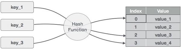
A hash table is a data structure that provides efficient insertion, deletion, and lookup operations on key-value pairs. It works by using a hash function to map each key to a position in an array, called the hash table, where the corresponding value is stored.
The hash function takes a key as input and generates a hash code, which is used to determine the position in the array where the value should be stored. Ideally, the hash function should distribute the keys uniformly across the hash table, to minimize collisions (i.e., when two or more keys map to the same position in the array).
To handle collisions, a hash table typically uses a collision resolution strategy, such as chaining or open addressing. Chaining involves storing all the values that hash to the same position in a linked list, while open addressing involves finding the next available position in the array to store the value.
One of the advantages of hash tables is their speed. In the average case, operations on a hash table have a constant-time complexity of \(O(1)\), meaning that the time taken to perform an operation does not depend on the size of the hash table. This makes hash tables ideal for applications where fast lookup and insertion times are important.
Overall, hash tables are an important data structure in computer science, and are widely used in applications such as databases, compilers, and web servers. However, the efficiency of hash tables depends on the quality of the hash function used, and collisions can still occur, which can degrade performance.
Storing data#
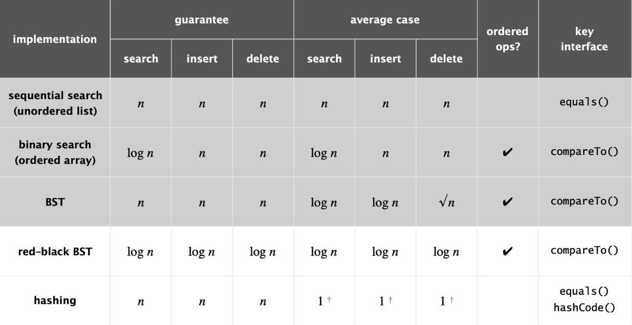
Fig. 66 Summary Table#
Hash Tables#
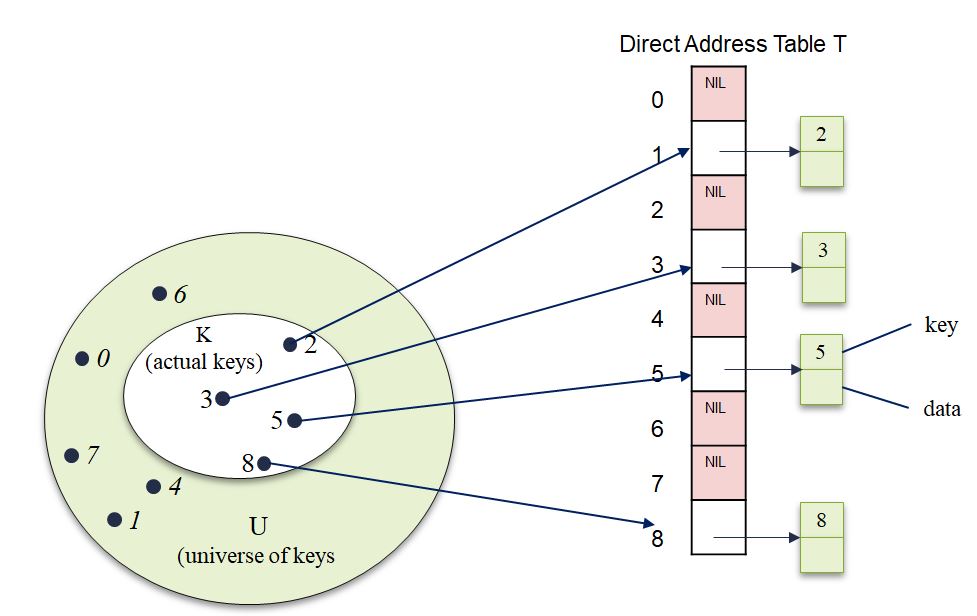
implements an associative array or dictionary
an abstract data type that maps keys to values
uses a hash function to compute an \(index\), also called a \(hash code\)
at lookup, the key is hashed and the resulting hash indicates where the corresponding value is stored.

Fig. 67 Hash Table#
Why not…#
Best-case \(O(1)\)
Practical limitations
Extra space
A given integer in a programmming language may not store \(n\) digits
Therefore, not always a viable option
Hash Functions#
a function converting a piece of data into a smaller, more practical integer
the integer value is used as the \(index\) between 0 and \(m-1\) for the data in the hash table
ideally, maps all keys to a unique slot \(index\) in the table
perfect hash functions may be difficult, but not impossible to create
Efficiently computable
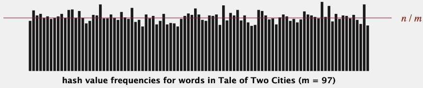
Should uniformly distribute the keys (each table position equally likely for each)
Should minimize collisions
Should have a low load factor \(\frac{\#\ items\ in\ table}{table\ size}\)
Modular Hashing#
\(h\) = hash function
\(x\) = key
\(HT\) = hash table
\(m\) = table size
\(b\) = buckets
\(r\) = items per bucket
Suppose there are six students:
\(a1, a2, a3, a4, a5, a6\) in the Data Structures class and their IDs are:
Suppose \(HT[b] \leftarrow a\)…
Uniform Hashing#
- Assumption#
Any key is equally likely (and independent of other keys) to hash to one of \(m\) possible indices
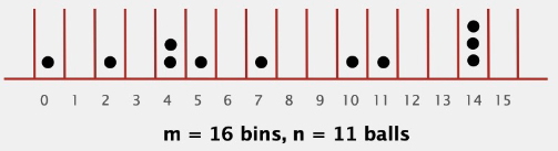
- Bins and Balls#
Toss \(n\) balls uniformly at random into \(m\) bins
- Bad News [birthday problem]#
In a random group of 23 people, more likely than not that two people share the same birthday Expect two balls in the same bin after \(\sim \sqrt{\pi * \frac{m}{2}} \ \ \ \ \ \ \ \ \ \ // = 23.9\ when\ m = 365\)
- Good News#
when \(n \gt\gt m\), expect most bins to have \(\approx \frac{n}{m}\) balls when \(n = m\), expect most loaded bin has \(\sim \frac{ln\ n}{ln\ ln\ n}\) balls
Collisions#
Two distinct keys that hash to the same index birthday problem
\(\Rightarrow\) can’t avoid collisions
load balancing
\(\Rightarrow\) no index gets too many collisions
\(\Rightarrow\) ok to scan though all colliding keys
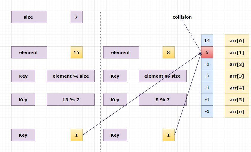
Fig. 68 collision#
Separate Chaining#
keeps a list of all elements that hash to the same value
Performance
\(m\) = Number of slots in hash table
\(n\) = Number of keys to be inserted in hash table
Load factor \(α = n/m\)
Expected time to search or delete = \(O(1 + α)\)
Time to insert = \(O(1)\)
Time complexity of search, insert, and delete is \(O(1)\ if\ α\ is\ O(1)\)
Example
\(h(k_1) = 0\ \ \ \ \%\ 10 = 0\ \ \ \ \ \ \ \Rightarrow\ \ \ \ \ HT[0] \leftarrow 0\)
\(h(k_2) = 81\ \ \%\ 10 = 1\ \ \ \ \ \ \ \Rightarrow\ \ \ \ \ HT[1] \leftarrow 81\)
\(h(k_3) = 64\ \ \%\ 10 = 4\ \ \ \ \ \ \ \Rightarrow\ \ \ \ \ HT[4] \leftarrow 64\)
\(h(k_4) = 25\ \ \%\ 10 = 5\ \ \ \ \ \ \ \Rightarrow\ \ \ \ \ HT[5] \leftarrow 25\)
\(h(k_5) = 36\ \ \%\ 10 = 6\ \ \ \ \ \ \ \Rightarrow\ \ \ \ \ HT[6] \leftarrow 36\)
\(h(k_6) = 49\ \ \%\ 10 = 9\ \ \ \ \ \ \ \Rightarrow\ \ \ \ \ HT[9] \leftarrow 49\)
\(h(k_7) = 1\ \ \ \ \%\ 10 = 1\ \ \ \ \ \ \ \Rightarrow\ \ \ \ \ HT[1] \leftarrow 1\)
\(h(k_8) = 4\ \ \ \ \%\ 10 = 4\ \ \ \ \ \ \ \Rightarrow\ \ \ \ \ HT[4] \leftarrow 4\)
\(h(k_9) = 16\ \ \%\ 10 = 6\ \ \ \ \ \ \ \Rightarrow\ \ \ \ \ HT[6] \leftarrow 16\)
\(h(k_{10}) = 9\ \ \ \%\ 10 = 9\ \ \ \ \ \ \ \Rightarrow\ \ \ \ \ HT[9] \leftarrow 9\)
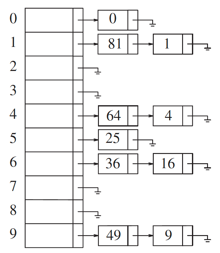
Fig. 69 A separate chaining hash table#
Advantages / Disadvantages??
Simple to implement.
Hash table never fills up, we can always add more elements to the chain.
Less sensitive to the hash function or load factors.
It is mostly used when it is unknown how many and how frequently keys may be inserted or deleted.
The cache performance of chaining is not good as keys are stored using a linked list. Open addressing provides better cache performance as everything is stored in the same table.
Wastage of Space (Some Parts of the hash table are never used)
If the chain becomes long, then search time can become O(n) in the worst case
Uses extra space for links
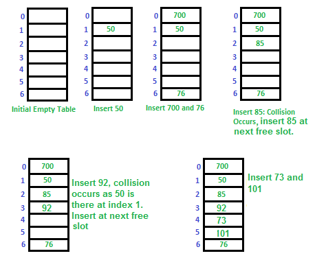
Open Addressing#
keeps a list of all elements that hash to the same value
\(h_i(x) = (Hash(x) + i) \ \% \ HashTableSize\)
If \(h_0(x) = (Hash(x) + 0) \ \% \ HashTableSize\)
If \(h_1(x) = (Hash(x) + 1) \ \% \ HashTableSize\)
If \(h_2(x) = (Hash(x) + 2) \ \% \ HashTableSize\)
… and so on
Quadratic Probing#
Double Hashing#
Rule
Example
\(Arr[0]\) |
\(700\) |
\(Arr[1]\) |
\(50\) |
\(Arr[2]\) |
|
\(Arr[3]\) |
|
\(Arr[4]\) |
|
\(Arr[5]\) |
|
\(Arr[6]\) |
\(76\) |
\(Arr[0]\) |
\(700\) |
\(Arr[1]\) |
\(50\) |
\(Arr[2]\) |
\(85\) |
\(Arr[3]\) |
|
\(Arr[4]\) |
|
\(Arr[5]\) |
|
\(Arr[6]\) |
\(76\) |
\(Arr[0]\) |
\(700\) |
\(Arr[1]\) |
\(50\) |
\(Arr[2]\) |
\(85\) |
\(Arr[3]\) |
\(92\) |
\(Arr[4]\) |
|
\(Arr[5]\) |
|
\(Arr[6]\) |
\(76\) |
\(Arr[0]\) |
\(700\) |
\(Arr[1]\) |
\(50\) |
\(Arr[2]\) |
\(85\) |
\(Arr[3]\) |
\(92\) |
\(Arr[4]\) |
|
\(Arr[5]\) |
\(73\) |
\(Arr[6]\) |
\(76\) |
\(Arr[0]\) |
\(700\) |
\(Arr[1]\) |
\(50\) |
\(Arr[2]\) |
\(85\) |
\(Arr[3]\) |
\(92\) |
\(Arr[4]\) |
\(101\) |
\(Arr[5]\) |
\(73\) |
\(Arr[6]\) |
\(76\) |
Comparison#
Easy to implement
Best cache performance
Suffers from clustering
Average cache performance
Suffers less from clustering
Poor cache performance
No clustering
Requires more computation time