Greedy Algorithms#
A greedy algorithm is a type of algorithmic approach that follows the “greedy” heuristic, which means it always makes the locally optimal choice at each step in the hope of finding a global optimum solution. In other words, it makes the best possible decision at each step based on the information available at that time, without considering the future consequences.
In data structures, greedy algorithms are often used for optimization problems where the goal is to find the best possible solution from a set of possible solutions. These algorithms are especially useful when there are many possible solutions and it’s difficult to find the best one through brute force methods.
Examples of greedy algorithms in data structures include:
Huffman coding, which is used for data compression
Kruskal’s algorithm, which is used to find the minimum spanning tree of a graph
Dijkstra’s algorithm, which is used to find the shortest path in a graph
Fractional knapsack problem, which is used to maximize the value of items in a knapsack with limited capacity.
Greedy algorithms can be simple and efficient, but they are not always optimal, and sometimes they can lead to suboptimal solutions. Therefore, it’s important to carefully analyze the problem and determine whether a greedy approach is appropriate.
Definition#
A greedy algorithm is an approach for solving a problem by selecting the best option available at the moment. It doesn’t worry whether the current best result will bring the overall optimal result.
The algorithm never reverses the earlier decision even if the choice is wrong. It works in a top-down approach.
This algorithm may not produce the best result for all the problems. It’s because it always goes for the local best choice to produce the global best result.
However, we can determine if the algorithm can be used with any problem if the problem has the following properties:
If an optimal solution to the problem can be found by choosing the best choice at each step without reconsidering the previous steps once chosen, the problem can be solved using a greedy approach. This property is called greedy choice property.
If the optimal overall solution to the problem corresponds to the optimal solution to its sub-problems, then the problem can be solved using a greedy approach. This property is called optimal substructure.
Advantages & Disadvantages#
Advantages
The greedy approach is easy to implement.
Typically have less time complexity.
Greedy algorithms can be used for optimization purposes or finding close to optimization in case of Hard problems.
The greedy approach can be very efficient, as it does not require exploring all possible solutions to the problem.
The greedy approach can provide a clear and easy-to-understand solution to a problem, as it follows a step-by-step process.
The solutions to subproblems can be stored in a table, which can be reused for similar problems.
– gfg
Disadvantages
The local optimal solution may not always be globally optimal.
Lack of proof of optimality.
The greedy approach is only applicable to problems that have the property of greedy-choice property meaning not all problems can be solved using this approach.
The greedy approach is not easily adaptable to changing problem conditions.
– gfg
Example#

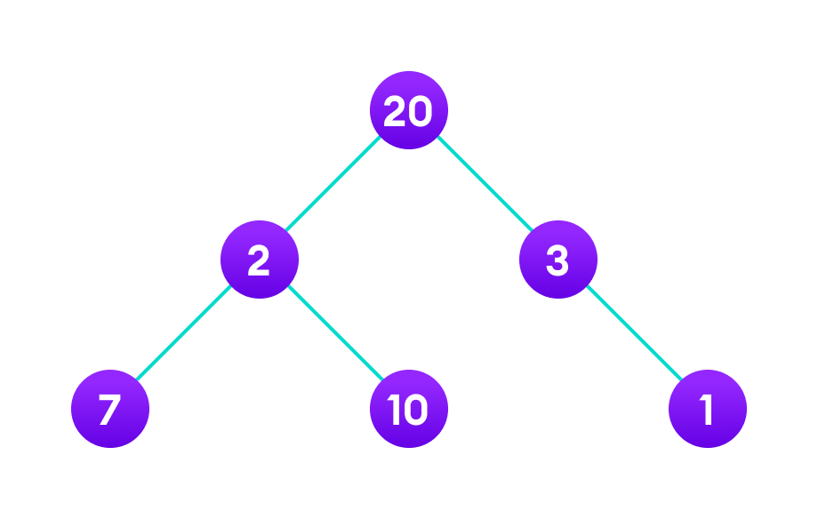
Fig. 107 Apply greedy approach to this tree to find the longest route#

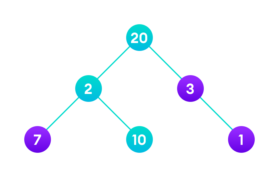
Fig. 108 longest path#
Let’s start with the root node \(20\). The weight of the right child is \(3\) and the weight of the left child is \(2\).
Our problem is to find the largest path. And, the optimal solution at the moment is \(3\). So, the greedy algorithm will choose \(3\).
Finally the weight of an only child of \(3\) is \(1\). This gives us our final result \(20 + 3 + 1 = 24\).
However, it is not the optimal solution. There is another path that carries more weight \((20 + 2 + 10 = 32)\).
Therefore, greedy algorithms do not always give an optimal/feasible solution.
Considerations#
Greedy algorithms make the locally optimal choice at each step, without considering the consequences of that choice on future steps.
Greedy algorithms can be used to solve optimization problems that can be divided into smaller sub-problems.
Greedy algorithms may not always find the optimal solution. It is important to prove the correctness of a greedy algorithm and to understand its limitations.
Greedy algorithms can be applied in many contexts, including scheduling, graph theory, and dynamic programming.
When designing a greedy algorithm, it is important to identify the optimal substructure and the greedy choice property.
The time complexity of a greedy algorithm depends on the specific problem and the implementation of the algorithm.
Greedy algorithms can sometimes be used as a heuristic approach to solve problems when the optimal solution is difficult to find in practice.
In some cases, a greedy algorithm may provide a solution that is close to the optimal solution, but not necessarily the exact optimal solution. These solutions are known as approximate solutions.
– gfg
Variances#
Greedy |
Divide & Conquer |
Dynamic Programming |
|---|---|---|
Optimises by making the best choice at the moment |
Optimises by breaking down a subproblem into simpler versions of itself and using multi-threading & recursion to solve |
Same as Divide and Conquer, but optimises by caching the answers to each subproblem as not to repeat the calculation twice. |
Doesn’t always find the optimal solution, but is very fast |
Always finds the optimal solution, but is slower than Greedy |
Always finds the optimal solution, but could be pointless on small datasets. |
Requires almost no memory |
Requires some memory to remember recursive calls |
Requires a lot of memory for memoisation / tabulation |
Pseudocode#
Basic structure of a greedy algorithm
function GreedyAlgorithm(problem) {

  // currentState = initial state of problem
  while (currentState != goalState) {
    nextState = chooseNextState(currentState);
    currentState = nextState;
  }

  return currentState;
}
The first step is to set the current state to the initial state of the problem.
Next, we keep looping until the current state is equal to the goal state. Inside the loop, we choose the next state that we want to move to. This is done by using a function calledchooseNextState().
Finally, we set the current state to be equal to the next state that we have just chosen and return to the goal state.
chooseNextState()
function chooseNextState(currentState) {
  // find all possible next states
  nextStates = findAllPossibleNextStates(currentState);

  // choose the next state that is closest to the goal state
  bestState = null;
  for (state in nextStates) {
    if (isCloserToGoal(state, bestState)) bestState = state;
  }
  return bestState; }
First, we find all of the possible next states that we could move to from the current state.
Next, we loop through all of the possible next states and compare each one to see if it is closer to the goal state than the best state that we have found so far.
If it is, then we set the best state to be equal to the new state.
Finally, we return the best state that we have found.
