
Basic Sorts (Analysis)#
Sorting is a fundamental problem in computer science, and it involves arranging a collection of data in a specific order. There are various sorting algorithms available that can be used to sort data in ascending or descending order based on a specific criterion.
Some of the most basic sorting algorithms include:
- Bubble Sort
It is a simple sorting algorithm that repeatedly compares adjacent elements and swaps them if they are in the wrong order. This algorithm has a time complexity of \(O(n^2)\).
- Insertion Sort
It is a simple sorting algorithm that works by inserting each element in its proper place in a sorted sub-array. This algorithm has a time complexity of \(O(n^2)\) but performs better than bubble sort for small data sets.
- Selection Sort
It is a sorting algorithm that repeatedly selects the smallest element from an unsorted sub-array and swaps it with the first element of the sub-array. This algorithm has a time complexity of \(O(n^2)\).
- Merge Sort
It is a divide-and-conquer sorting algorithm that recursively divides the input array into two halves, sorts them separately, and then merges them back together. This algorithm has a time complexity of \(O(n\ log\ n\)\).
- Quick Sort
It is also a divide-and-conquer sorting algorithm that picks a pivot element and partitions the array around it. This algorithm has a time complexity of \(O(n\ log\ n)\) on average but can degrade to \(O(n^2)\) in the worst-case scenario.
Each sorting algorithm has its advantages and disadvantages in terms of time and space complexity, stability, adaptability, and implementation complexity. Understanding and comparing the different sorting algorithms is an important skill for anyone studying data structures and algorithms as it enables them to select the best algorithm for their use case.
Internships & Jobs#
Worst-case, Average-case, Best-case#
Analyze this code
 1unsigned int argmin (const std::vector<int> &values) {
 2    unsigned int length = values.size();
 3    assert(length > 0);
 4    unsigned int idx = 0;
 5    int current = values[0];
 6    for (unsigned int i = 1; i < length; i++) {
 7        if (values[i] < current) {
 8            current = values[i];
 9            idx = i;
10        }
11    }
12    return idx;
13}
\(T(n)\ =\ ?\)
\(based\ on\ number\ of\ comparisons\)
The number of comparisons in this program is n - 1, where n is the size of the vector.
Analyze this code
 1bool argk (const std::vector<int> &values,
 2                                    int k,
 3                        unsigned int &idx)
 4{
 5    unsigned int length = values.size();
 6    for (unsigned int i = 0; i < length; i++) {
 7        if (values[i] == k) {
 8            idx = i;
 9            return true;
10        }
11    }
12    return false;
13}
\(T(n)\ =\ ?\)
\(based\ on\ number\ of\ comparisons\)
The number of comparisons in this program is equal to the number of elements in the given vector. Therefore, the number of comparisons is dependent on the size of the input vector. The time complexity of this program is O(n), where n is the size of the input vector.
Analysis types#
😕 Worst-case
maximum time of algorithm on any input
🤔 Average-case
expected time of algorithm over all inputs
🦄 Best-case
minimum time of algorithm on some (optimal) input
Note
While asymptotic analysis describes \(T(n) \Rightarrow \infty\)…
asymptotic notation: big-O, big-\(\Omega\), \(\Theta\)
Case analysis looks into the different input types
best-case, worst-case, average-case
Examples#
1// pseudocode
2
3function factorial(n):
4    if n <= 1:
5        return 1
6    result = 1
7    for i in range(1, n+1):
8        result *= i
9    return result
❓Case
🤔 Best-case
Without possibility of extra steps, the only analysis can be best-case…
1// pseudocode
2
3function find_first(items, target):
4    index = 0
5    while index < len(items):
6        if items[index] == target:
7            return index
8        index += 1
9    return -1
❓Case
🤔 Average-case
Arguably, the first occurrence could be the first or last element/node in the collection. The majority of the time, it will not be either first or last, leading to only one logical result, average-case…
1// pseudocode
2
3function find_last(items, target):
4    index = len(items) - 1
5    while index >= 0:
6        if items[index] == target:
7            return index
8        index -= 1
9    return -1
❓Case
🤔 Worst-case
Arguably, the value could be found at anywhere but the last element/node of the collection. However, we must still complete a comparison of the desired value and each element/node in the collection to exhaust all possibilities, therefore, it would fall into worst-case…
Basic Sorting Algorithms#
Sorting#
Given \(n\) elements that can be compared according to a total order relation
we want to rearrange them in non-increasing/non-decreasing order
for example (non-decreasing):
input: sequence of items \(\ \ \ \ \ \ \ \ \ \ \ A = [k_0, k_1, \dots, k_{n - 1}]\)output: permutation of A \(\ \ \ \ \ \ \ \ \ \ \ B\ |\ B[0]\ \le\ B[1]\ \le \dots B[n - 1]\)
Insertion Sort#
Defined as…
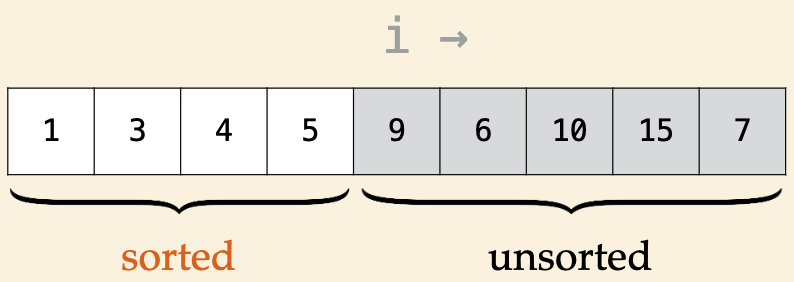
Array is divided into sorted and unsorted parts
algorithm scans array from left to right
Invariants
elements in sorted are in ascending order
elements in unsorted have not been seen
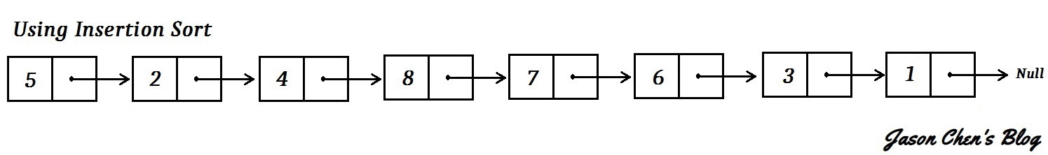
visualization : linked list
visualization : interactive
 1void insertion_sort(int* items, int size) {
 2    //grows the left part (sorted)
 3    for (int i = 1; i < size; i++) {
 4        int j = i;
 5        //inserts j in sorted part
 6        while (j > 0 && items[j-1] > items[j]) {
 7            swap(items[j-1], items[j]);
 8            j--;
 9        }
10    }
11}
Analysis — Insertion Sort(comparisons)#
Running time depends on the input
- Worst-case?#
input is already sorted in descending order
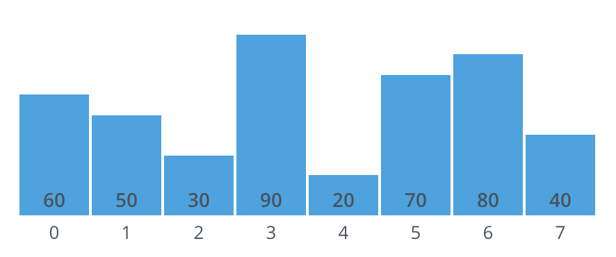
- Average-case?#
each element \(\approx\) halfway order
expect every element to move \(O(\frac{n}{2})\) times
- Best-case?#
input is already sorted in ascending order
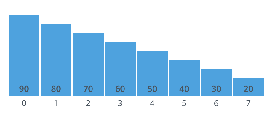
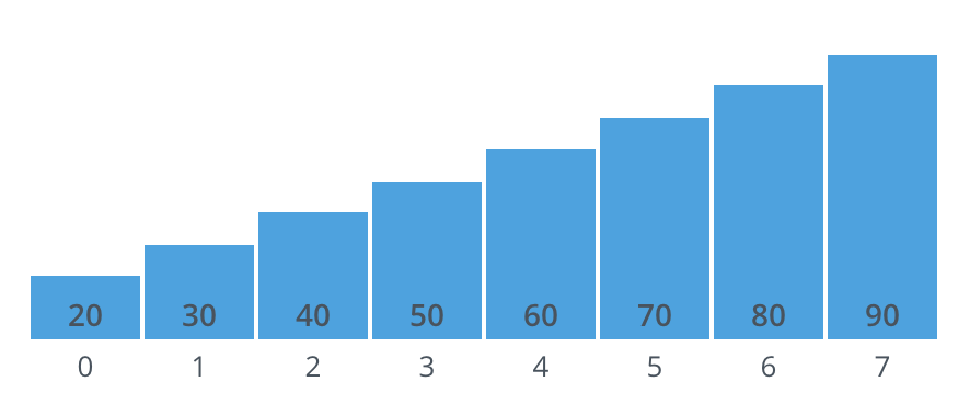
{90, 80, 70, 60, 50, 40, 30, 20}
{60, 50, 30, 90, 20, 70, 80, 40}
{20, 30, 40, 50, 60, 70, 80, 90}
Partially sorted arrays#
A pair of keys that are out of order
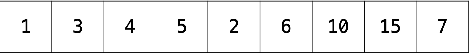
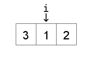
Fig. 95 swapping indices#
“array is partially sorted if the number of pairs that are out-of-order is \(O(n)\)”
For partially-sorted arrays, insertion sort runs in linear time.
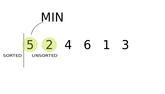
Selection Sort#
Defined as
Array is divided into sorted and unsorted parts
algorithm scans array from left to right
Invariants
elements in sorted are fixed and in ascending order
no element in unsorted is smaller than any element in sorted
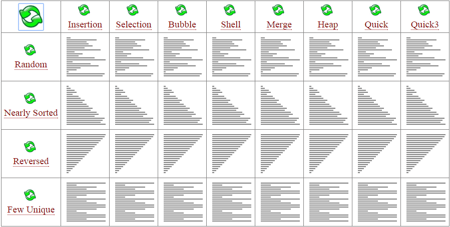
visualization : gif

visualization : interactive
 1void selectionsort (int *A, unsigned int n) {
 2    int temp;
 3    unsigned int i, j, min;
 4    // grows the left part (sorted)
 5    for (i = 0; i < n; i++) {
 6        min = i;
 7        // find min in unsorted part
 8        for (j = i + 1; j < n; j++) {
 9            if (A[j] < A[min]) {
10                min = j;
11            }
12        }
13        // swap A[i] and A[min]
14        temp = A[i];
15        A[i] = A[min];
16        A[min] = temp;
17    }
18}
\(Number\ of\ comparisons?\ |\ Number\ of\ exchanges?\)
In the above snippet, the selection sort algorithm is implemented. The number of comparisons and exchanges made depend on the size of the input array n.
For comparisons, there are two nested for-loops that compare all elements of the array. The outer for-loop, which runs from \(i = 0\) to \(n - 1\), runs n times. The inner for-loop, which runs from \(j = i + 1\) to \(n - 1\), runs \(n - i - 1\) times. Therefore, the total number of comparisons is:
For exchanges, each iteration of the outer for-loop swaps the element at index i with the element at index min. Since this occurs n times, the total number of exchanges is n.
visualization : comparisons & exchanges
Notes
Selection Sort: moves through each element finding the minimum value and replacing the current element value as it goes.
sorted portion left order, fixed, untouched
unsorted iterated through to find remaining min value to swap current element value
Summary#
Best-Case |
Average-Case |
Worst-Case |
|
|---|---|---|---|
Selection Sort |
|||
Insertion Sort |
Best-Case |
Average-Case |
Worst-Case |
|
|---|---|---|---|
Selection Sort |
\(O(n^2)\) |
\(O(n^2)\) |
\(O(n^2)\) |
Insertion Sort |
\(O(n)\) |
\(O(n^2)\) |
\(O(n^2)\) |